3. Tooling From First Principles — None of This is New
“There is nothing new except what has been forgotten.” — Marie Antoinette
As IT architects, we work hard to make sure that our ideas are easy to understand and, therefore, learned many years ago that visual representation can be much more powerful than the written word. As a result, much of what we do is visual, and when we first document our ideas, we metaphorically apply broad brush strokes to outline the essential technical elements necessary. This is how and why the likes of Context Diagrams and Architectural Overviews come about, both of which comprise little more than a collection of drawn boxes, connected using a series of lines. That is why some experts talk of IT architects only needing two weapons — the shield and the spear.
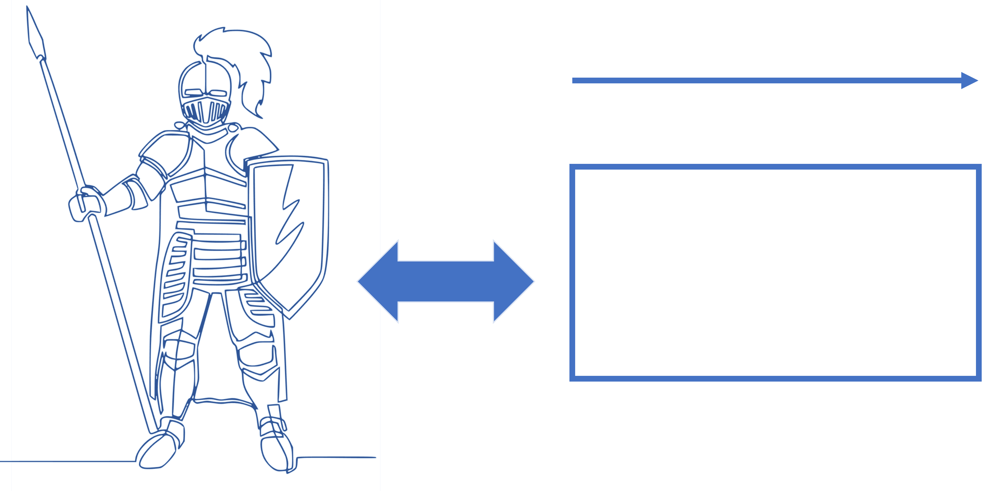
Here, the shield is analogous to box notation and, likewise, the spear represents the various types of connection used in architectural schematics. All that matters in such diagrams is that the things or ideas needing representation are communicated through the drawing of boxes or similar shapes. Likewise, the connections between these things are shown through the drafting of connecting lines. Both boxes and lines can then be labeled and/or annotated to bring their contribution to any overarching narrative to life. In that way, structure is added to the processes involved in architectural thinking, so that large problems (of less than a headful) can be broken down into smaller and much easier units to handle; see Figure 4.
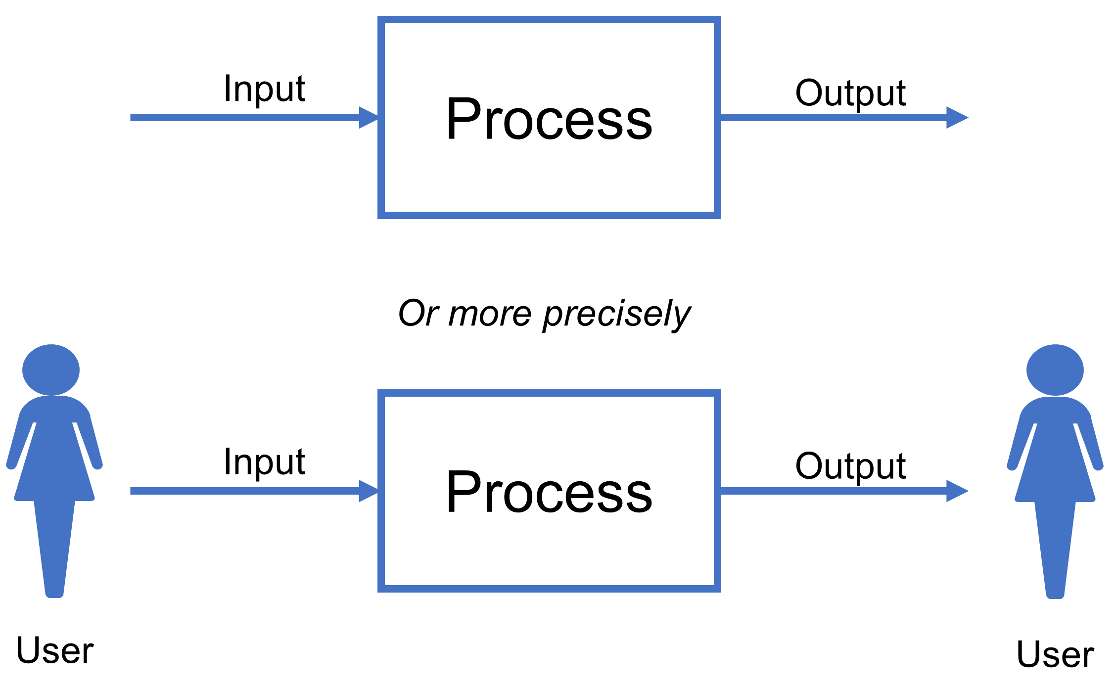
In any given architectural diagram then, whether logical or physical, boxes of various sorts are invariably related to other boxes through a single, or multiple, lines. For instance, when a line is used to depict the movement or exchange of data between two processes, in the form of boxes, any implementation details associated with that transfer might be separated out and described via a further schematic or some form of additional narrative. This helps to simplify the diagram, so that specific points can be made, abstractions upheld, and a clear separation of concerns maintained.
Once the general composition of boxes and lines has been worked through, things do not change all that much, regardless of whatever viewpoint needs representing. So, different shapes and lines can be swapped in and out as necessary to get across what is important. Whichever way, the loose idea (nomenclature) of boxes and lines always lies beneath. For instance, when using conventions embodied in the Unified Modeling Language™ (UML®) standard, boxes and lines of various kinds can be composed to form a range of diagrams, two examples of which are shown in Figure 5.[1]
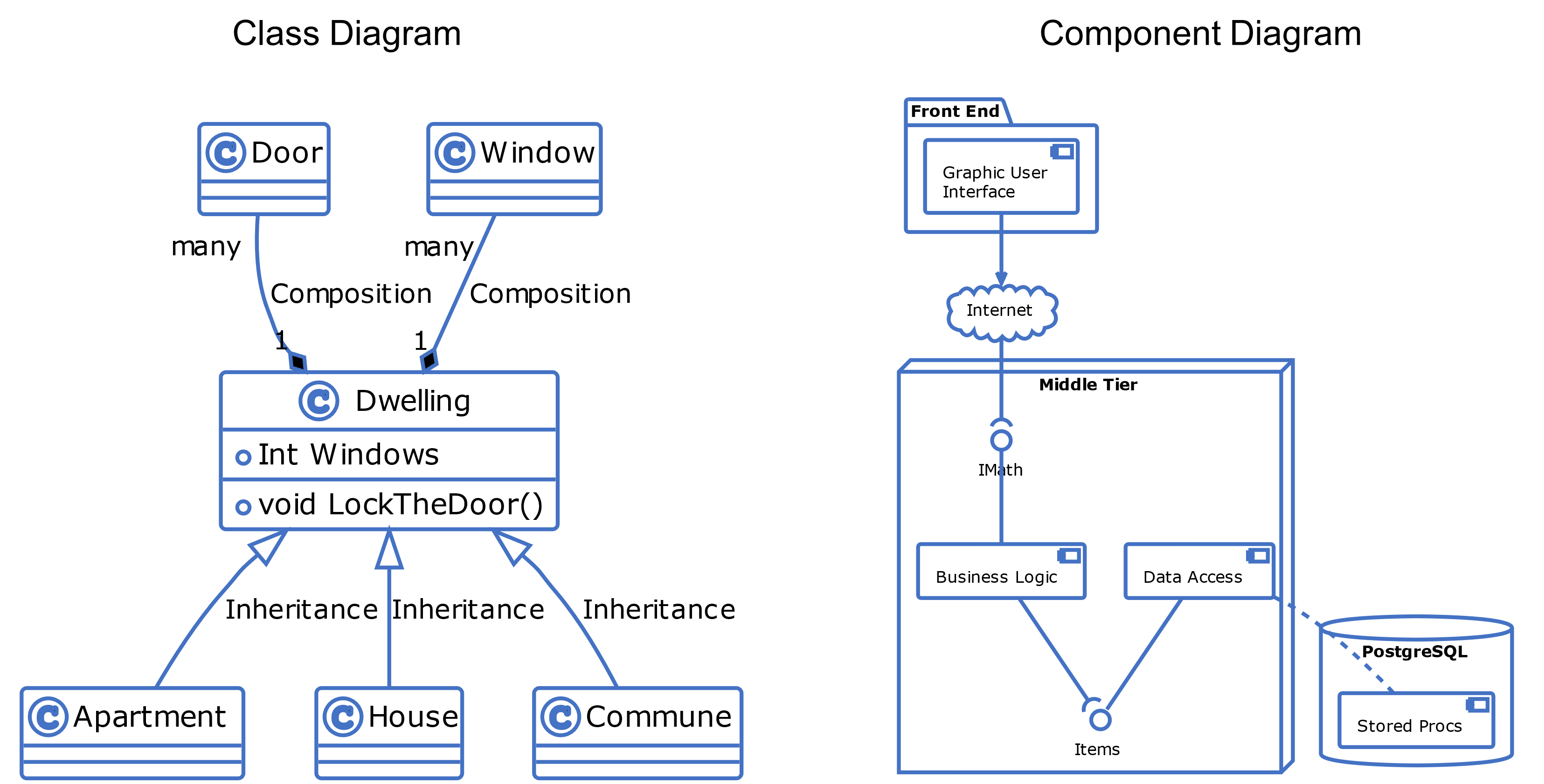
The point to note is that whatever framework is used, its diagrammatic expression is singularly limited by the range of shapes and lines listed within the vocabularies of its various standards.
More formally, the shapes and lines involved in any design standard function as a finite set of abstract types, aimed at supporting the communication of architectural intent; that is, they only cover the things that need to be said. They do not, however, have anything foundational to say about how such things might be brought together to create wholesome descriptions of that intent. That guidance is provided through architectural practice, often referred to as “methodology”, embodied elsewhere within the framework. In that way, various shapes and lines can be plugged together to give us the useful tools and methods we know and love as IT architects.
Once complete, the diagrams produced hopefully model all the salient characteristics of some architectural aspect, important to the problem space being considered, and, for that reason, they themselves become known as Models. Out of that comes the discipline we now know as Model Driven Architecture® (MDA®).
3.1. Model Driven Architecture
MDA is a software and systems development approach which emphasizes the importance of models in the development process. It therefore defines a set of guidelines for creating models that describe different aspects of an IT system, such as its functionality, structure, and behavior. These models can then be used to generate code, documentation, and other artifacts.
The key components of MDA can be seen as:
-
Platform Independent Models (PIM)
These provide abstract representations of the system under consideration that are independent of any particular implementation technology or platform. PIMs, therefore, represent an IT system’s functionality and behavior in a way that can be understood by both technical and non-technical stakeholders. -
Platform Specific Models (PSM)
These model-specific details of how a PIM will be implemented on a particular platform. PSMs, therefore, define the specific technologies, languages, and tools to be used when building and deploying build an IT system. -
Model Transformations
These define the process used to automatically generate code, documentation, and other artifacts from PIMs and PSMs. Model transformation, therefore, is facilitated by tools that can analyze these models and generate appropriate codified outputs.
Consequently, MDA specifically promotes the separation of concerns between the different aspects of a software system, thereby allowing developers to focus on each aspect independently. This separation also enables IT systems to be developed using different technologies and platforms, making them more adaptable and future-proof. This leads to a key benefit, in that MDA has the ability to improve the efficiency and consistency of development and deployment processes. By using models to describe an IT system, developers can quickly and accurately communicate the system’s requirements and design to stakeholders. Additionally, the use of model transformations can significantly reduce the amount of manual coding required, which, in turn, can potentially reduce errors and lead to productivity gains.
3.2. Toward an Ecosystems Framework
Approaches like MDA are not a panacea for the effective design and delivery of all IT systems though. They have drawbacks, and these unfortunately become clear when working at hyper-enterprise scales. Indeed, many of MDA’s strengths work to its detriment as the scale of the tasks it is being asked to address increase.
The first weakness unfortunately comes from MDAs defining strength, in that it was designed from the ground up to appeal to human users. That is why it is inherently graphical and intentionally reductionist in nature.
As a race, we evolved from the plains of Africa primarily on the strength of our flight or fight response. As such, our senses subconsciously prioritize inputs while our brains automatically filter out unnecessary signals. That leaves room for little more than the essentials of higher-level cognition. In a nutshell, that makes us sense-making survival machines, primed for life in a cave dweller’s world. As a result, and no matter how much we shout about it, the fineries of humanity’s historic achievements amount to little more than icing on that cake. For all that MDA works admirably as a coping mechanism to help when constructing modern-day IT systems, its value pales into insignificance when compared to the hardwired coping systems we have evolved over the millennia. That is why MDA is so effective; simply because it can help boil complex problems down into simple and static graphics which naturally appeal to our biological bias for visual stimuli. No more, no less.
But here is the thing. The world is not simple, and the more grandiose things get, generally the more simplicity is squeezed out. Detail abounds and important detail at that. It abounds, collects, and changes in a mix of evolving dependence and independence; a mix that often the human brain just cannot cope with, and which bounces off any attempt to reduce and simplify in human terms. Modern computers, however, now that is a whole other story. They simply thrive on detail. Where the human brain will prioritize, filter out, and overflow, today’s computer systems, with their multipronged AI, will just lap things up. Increasingly they do not even need to reduce or separate out the complex concerns that would have once floored their weaker ancestors. Complexity and scale, to them at least, amount to little more than an incremental list of work to do. It is about completing additional cycles and hardware configuration, that is all. The bigger the problem, the larger the infrastructure manifest needed and the longer we humans need to stand by the coffee machine awaiting our answers.
It is similar to the field of mathematics, where shapes and lines work well when we humans use them to help solve small and simple problems. The need to continually add more graphics to any workspace just overpowers as scale and complexity rise. Mathematics, on the other hand, fairly welcomes in scale and complexity. If you want to ramp things up or juggle more balls at the same time, that is a relatively easy thing for mathematics to do. Within, it embodies various types of containers[2] that do not care about how much data they are given. Indeed, their design is based on overcoming such obstacles. For them, managing size and complexity are mere arbitrary challenges only rattled by unruly concepts like infinity.
So, where does this leave us?
For IT architects to work effectively within this complex mix of detail and change at hyper-enterprise scale, at least two things need to be achieved. First is the broad acceptance that hyper-Enterprise Architectural challenges are indeed real and are materially different from all that has gone before. Beyond that, a framework, or frameworks, of extension to existing practice and a handful of new ideas are needed to help lay the ground for pragmatic progress. In truth though, few new ideas are really needed. All that is really required is a dust down of one or two foundational concepts and their reintroduction alongside modern-day architectural practice.
3.3. Graph Theory and Graphs
But how might these things be achieved? How might we distill and capture such extensions?
Hopefully, the answer should be clear. Hopefully, we are heading for a place where graphical representation and mathematical formality are both equally at home. Hopefully, that sweet spot can also accommodate change and chance at scale, so that we might model large, complex systems over many, many headfuls. And perhaps, just perhaps, that sweet spot will further align with the principles of existing architectural approaches like MDA?
Clearly the answer is “yes”.
In saying that, it is perhaps worth remembering that the relative informalities of approaches like MDA are themselves founded on some very formal mathematical thinking. Just connecting two shapes together via some form of line, for instance, rather handily provides a metaphor for the notion of set intersection [69] in set theory [70] — in that both shapes connect through some shared interest or trait. In that regard then, most of that which we consider as being informal in approaches like MDA, and more specifically in methodologies like UML perhaps, merely act as a façade over some altogether more formal thinking. Our methodologies then, no matter how formal or informal, provide gateways between that which is deeply philosophical and that which feels deeply familiar. They provide the wrapping that hides mathematics from everyday working practice, and so mathematics is, and always has been at home in the world of IT architecture. Likewise, the plug-and-play graphical nature of MDA is itself based on an independent and underlying mathematical model. That seeks to understand how ideas, things, events, and places, and so on might be connected into networks, and comes out of a group of mathematical ideas collectively known as graph theory [71] [72]. In that way, any schematic, representation or description that explicitly connects two or more things together in an abstract sense can be understood as a graph.
The basic idea of graphs was first introduced in the 18th century by the Swiss mathematician Leonhard Euler and is normally associated with his efforts to solve the famous Königsberg Bridge problem [73], as shown in Figure 6.[3]
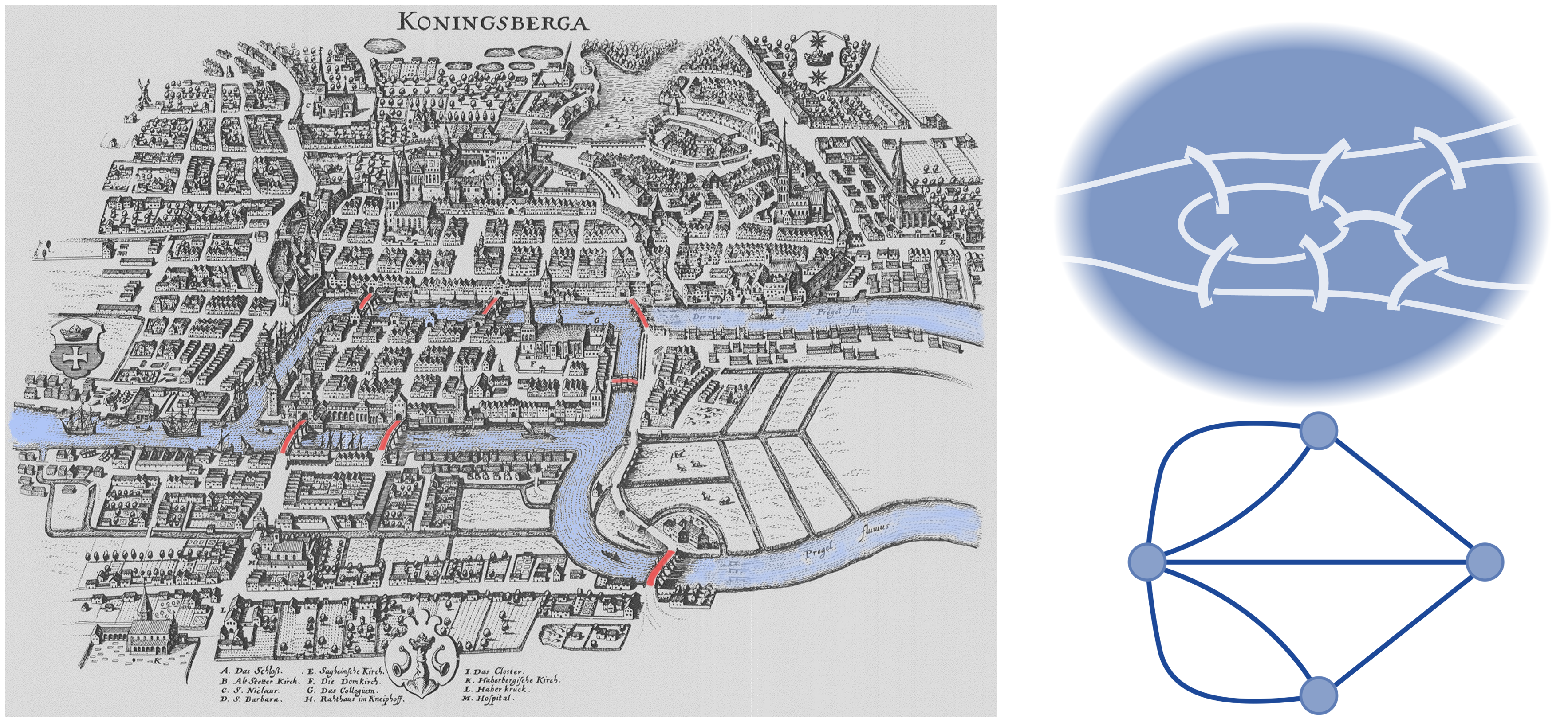
Previously known as Königsberg, but now known as Kaliningrad in Russia, the city sits on the south eastern corner of the Baltic Sea and was then made up of four land masses connected by a total of seven bridges. The question, therefore, troubling Euler was whether it might be possible to walk through the town by crossing each bridge just once?
In finding his answer, Euler astutely recognized that most of the city’s detail was superfluous to his challenge, so he set about focusing solely on the sites he needed to reach and the bridges he needed to cross to get between them. In doing that, he abstracted away from the immediate scenery and formed a simple map in his mind. When all but the essential detail was gone, what remained amounted to a collection of dots representing his essential locations, and seven lines representing the very bare minimum journey needed between them. In essence, he had created an abstract topology of the city consisting of mere dots and connecting lines. Each could be documented, of course, to name it as a specific place or route on his journey across the city, but in its most basic form, Euler had found a way of distilling out a problem’s all but necessary parts and glueing them together to give a coherent overall picture of a desired outcome. This abstract arrangement of dots and lines is what mathematicians today know today as an Undirected Graph (UG). By adding arrowheads to the lines involved, any such graph provides instruction to the reader, asking them to read it in a specific order, thereby making it a Directed Graph (DG) — of which Euler’s solution to the Königsberg Bridge problem provides an example. Beyond that, there is just one further type of graph worth mentioning for now, in a Directed Acyclic Graph (DAG). This is the same as a directed graph, but where the path of its connections never returns to previously visited ground. Figure 7 shows examples of the various types of graph.
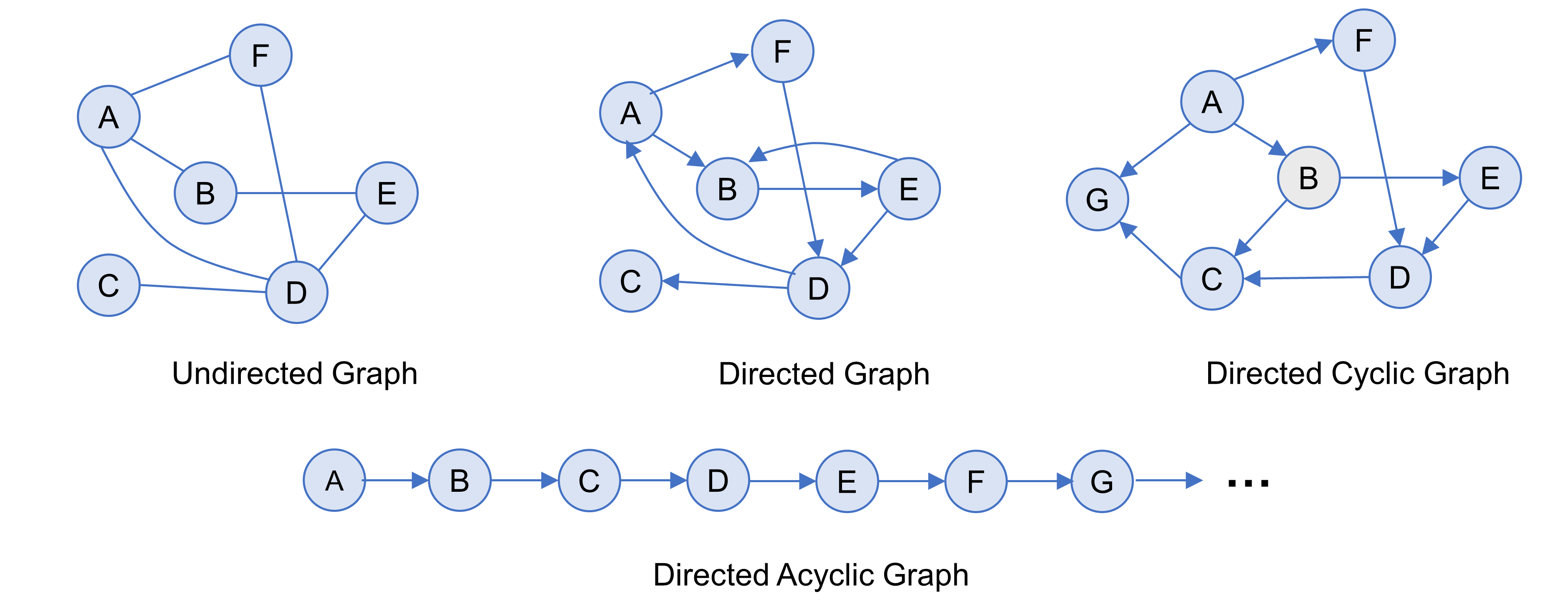
Graphs are therefore mathematical structures that model pairwise relations between points of interest (more formally known as nodes), as in the labeled circles shown in Figure 7. These nodes are then connected by lines (more formally known as arcs or edges) when a relationship is present. Nodes can also have relations with themselves, otherwise known as a self-loop [75].
3.4. Graphs, Architectural Schematics, and Semantic Extensibility
For hopefully now obvious reasons, graphs are especially useful in the field of IT architecture, simply because all the schematics that we, as IT architects, create (regardless of how formal or informal they might be), share, and trade, no matter what size, complexity, denomination, or related value, can be redrawn in pure graph form. That is all of them, regardless of whether they relate to structure or behavior, be that logical or physical. It really does not matter. That is because all such schematics possess graph structure under the hood. Graph theory, therefore, provides the common denominator across all architectural needs to describe and communicate[4] intent. Understanding graph theory consequently unlocks the logic that our world was built on.
Pick a Component Model, for instance. To redraw it as a pure graph, comprising of just dots and lines, is easy, in that the task simply becomes the same as drawing with the usual specialized shapes, but instead replacing them with generic nodes and arcs. All that is needed in addition is the overlaying of annotation, so that the schematic’s constituent elements can be identified uniquely and associated with the required specialized types, attributes, and so on. In that way, graph nodes can arbitrarily be listed as being of type component, chicken, waffle, or whatever. It is also the same with connecting arcs, so much so that mathematics even lists a specific type of graph, often referred to as a labeled or sometimes a weighted graph, that explicitly requires the adding of arc annotation for a graph to make complete sense.
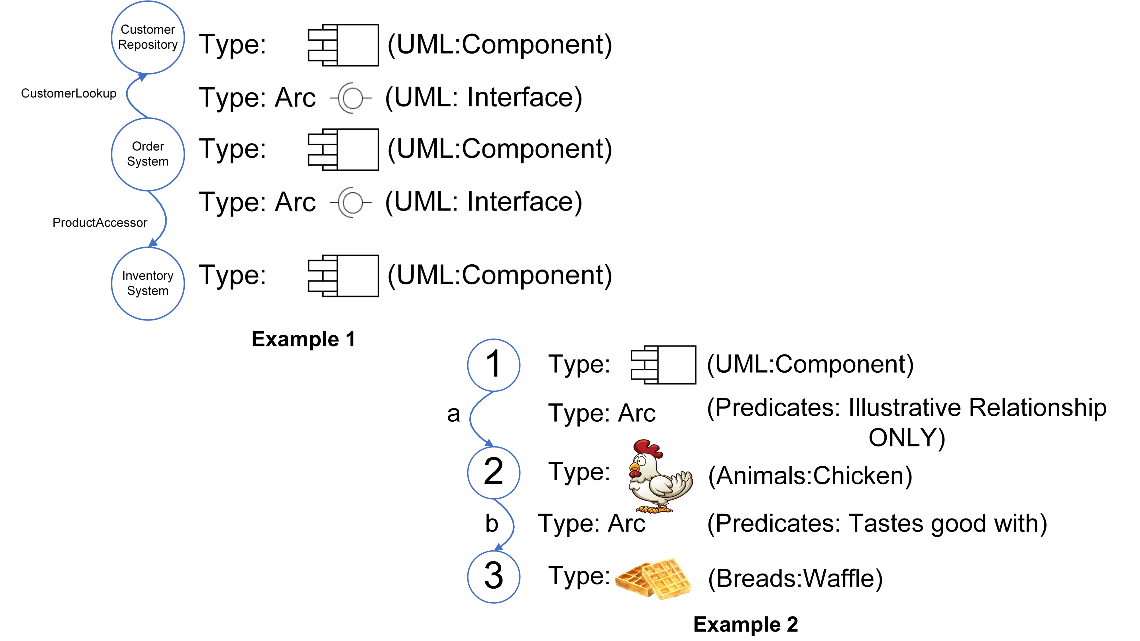
Figure 8 illustrates a couple of trivial graph examples, with the schematic on the left (Example 1) showing how a simple UML component model might be redrawn as a directed graph, and the diagram on the right (Example 2) illustrating that graphs are quite at home mixing up concepts from different frames of reference, methodologies, or whatever you will. As you will likely have already guessed, the “:” nomenclature used is for separating out the frame of reference (more formally known as vocabulary) used to contain each type and the named instance of that type. In that way, a graph node of overlaid type instance UML:Component calls out the use of a UML component type, and that it therefore complies with all the constraints and characteristics outlined within the UML standard for components. Likewise, the use of Animals:Chicken tells us that we are talking about a type of animal commonly known as “Chicken”. In both cases, the graph nodes are specifically referring to a single instance of both types. That is one UML:Component component and one Animals:Chicken chicken. Note also, that as where UML:Component relates to a very specific description of how to perceive and use the idea of a component, there is no such precise definition for Animals:Chicken implied here. For all that we might instinctively make the association with that type and our clucking feathered friends in the natural world, there is no absolute association at this point. Therefore, without a concrete definition of a vocabulary and its terms in place (as is the case with UML), the meaning (more formally known as semantics) associated with any given element within a graph cannot be precisely ascertained. That precision must be documented externally to the graph itself and referenced existentially before the actual intent behind a graph’s composition can be properly understood.
3.5. Applying Measurement Systems to Graph Context
There is, however, another way to draw the previous graphs.[5]
Let us take the Component-Chicken-Waffle example and this time frame it a bit better; that is, let us imagine that the ideas involved live in an imaginary space in our mind. This is the place where we bring together all the UML Types, Animals, and Breads that we know — sort of a smashed together list of all the things relevant across all three areas, if you like. In doing that, we can mark out that space evenly, so that it resembles a map of sorts, in much the same way that we often flatten out a physical landscape into a pictorial representation. After that, we can start to plot the various elements needed within our problem space, as shown in Figure 9.
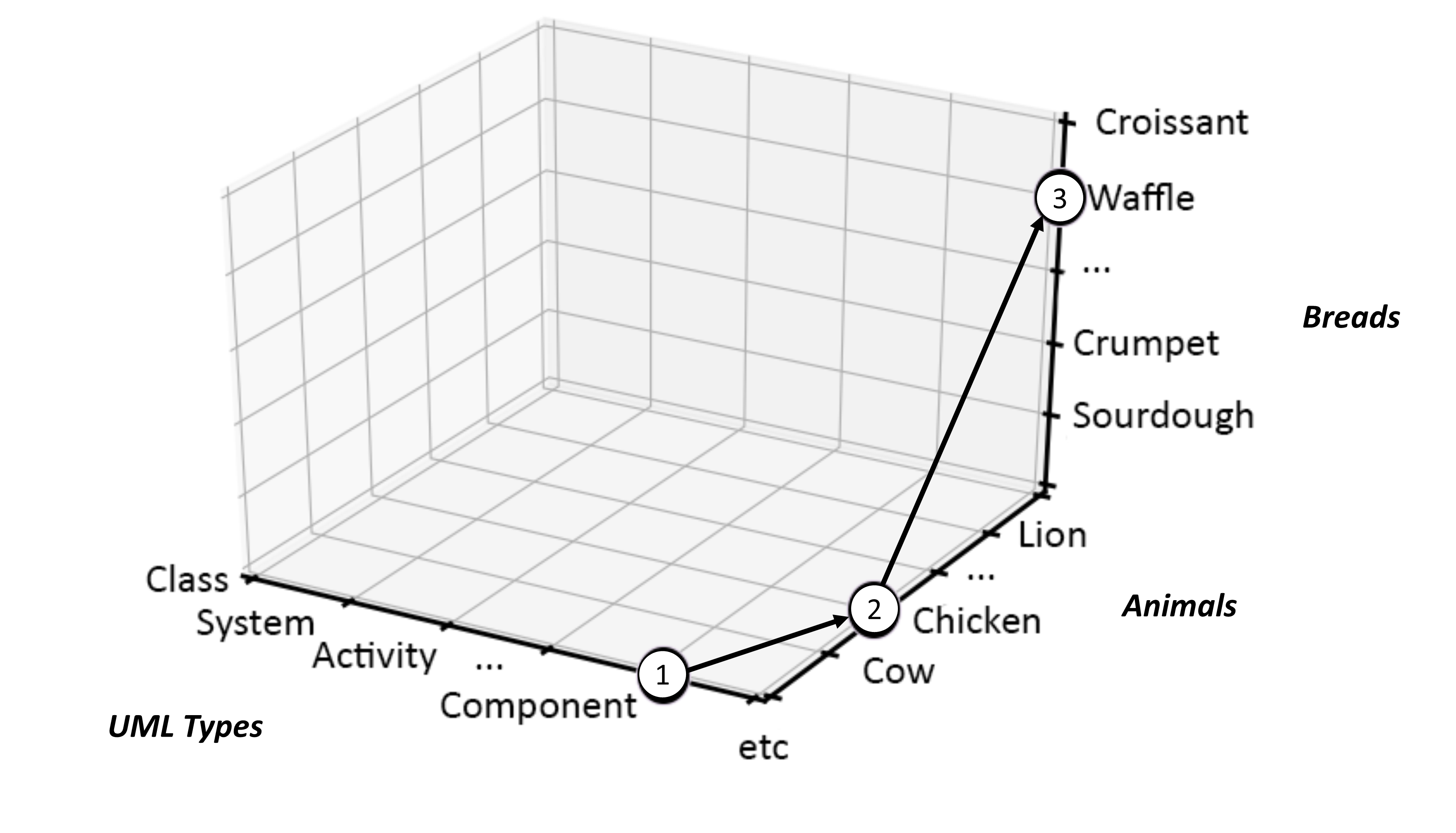
This “framing” actually brings two types of graph together; the first being the graph formalism described in Figure 8, which contains nothing more than nodes connected by arcs. The second, however, might feel more familiar to you, as it is the one taught in schools to draw out bar charts, histograms, line graphs, and the like. This type of graph is what mathematicians like to refer to as a Cartesian Graph or more properly a Cartesian Coordinate space or system [76]. In school, you were likely taught this by drawing two-dimensional X,Y graphs, in which two values can be plotted together to show some shared property in a two-dimensional space. But in Figure 9 we are using three dimensions to map onto the three ideas needing representation in our example.
With all that in mind, it becomes possible to make sense of Figure 9. In basic terms, it says that we are firstly dealing with a single thing or idea that is all about UML Components and not at all about Animals or Breads. Likewise, we are also dealing with a single thing or idea that is concerned with Animals and not at all about UML Types or Breads. Lastly, we are dealing with a thing or idea that is all about Breads and not at all about either UML Types or Animals. This then places our Component-Chicken-Waffle graph inside a Cartesian coordinate space, which in turn provides a measurement system allowing us to compare and contrast anything we place within it.
This is a very powerful idea, not only because it allows us to precisely pin down what we need to talk about, but it also allows us to blur the lines between the things needing representation. In that way, it is perfectly legitimate to talk about a concept requiring various degrees of chicken and waffle together, perhaps like a delicious breakfast, as shown in Figure 10.
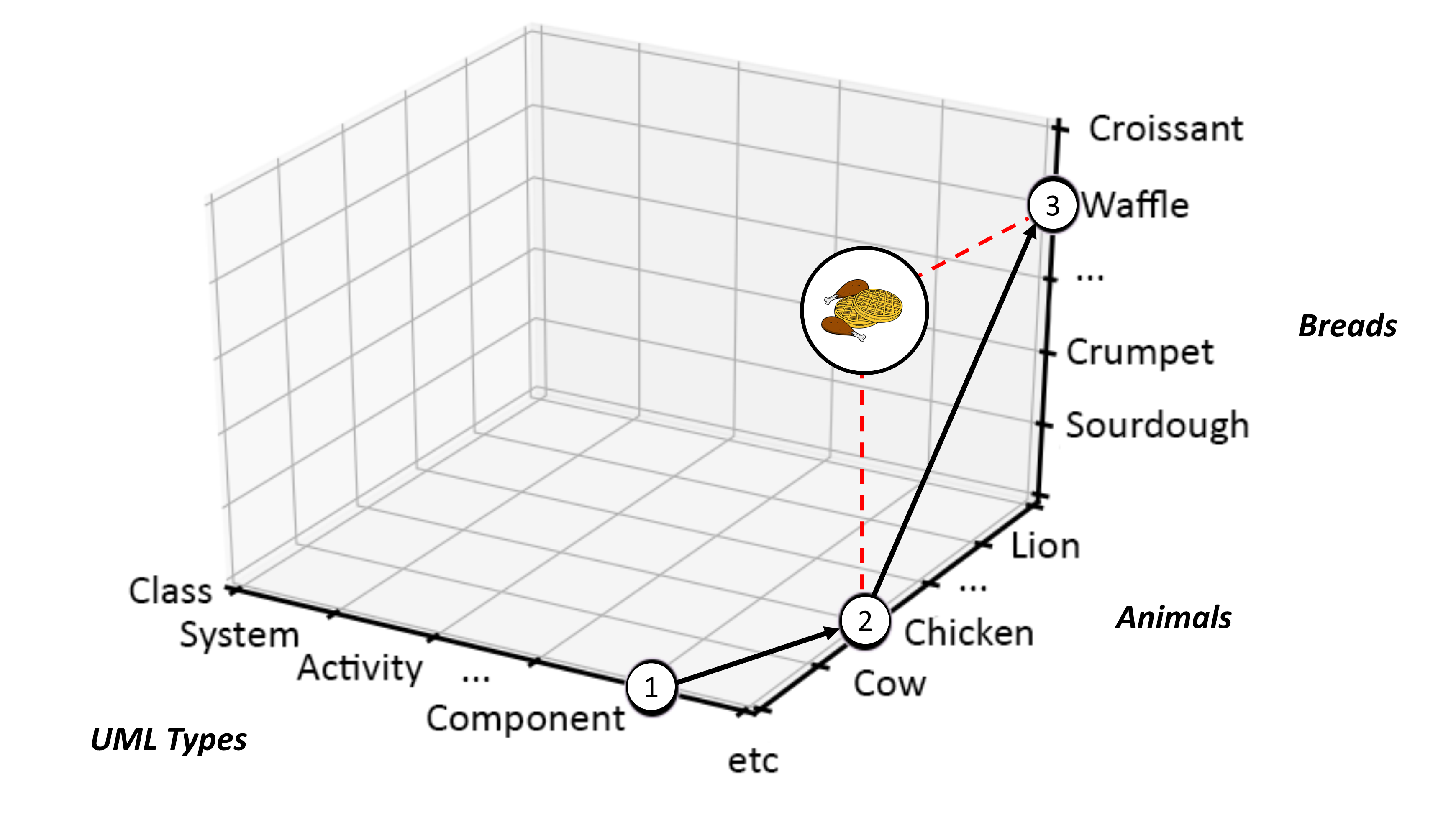
Notice here that the newly added breakfast node (linked using red dashed lines) contains no element of type UML:Component, no doubt that is because UML Components are not very tasty or are not on the breakfast menu! That is not a joke. It is a matter of precise and formal semantic denotation.[6] Nevertheless, speaking of taste, why don’t we consider not only assigning a specific type to each of our graph nodes, but further think about type as just one of any number of potentially assignable attributes, Succulence and maybe Deliciousness being others. If that were indeed so, then succulence and deliciousness would lie on a sliding, or continuous, scale, whereas, with type, we would normally consider things as being discretely of type, or not — as in an all or nothing classification.
In truth, however, both scales turn out to be continuous, as discrete measurement turns out to simply be a special form of continuous assessment, using especially course units between relevant points of measurement.
3.6. Continuous Cartesian Spaces
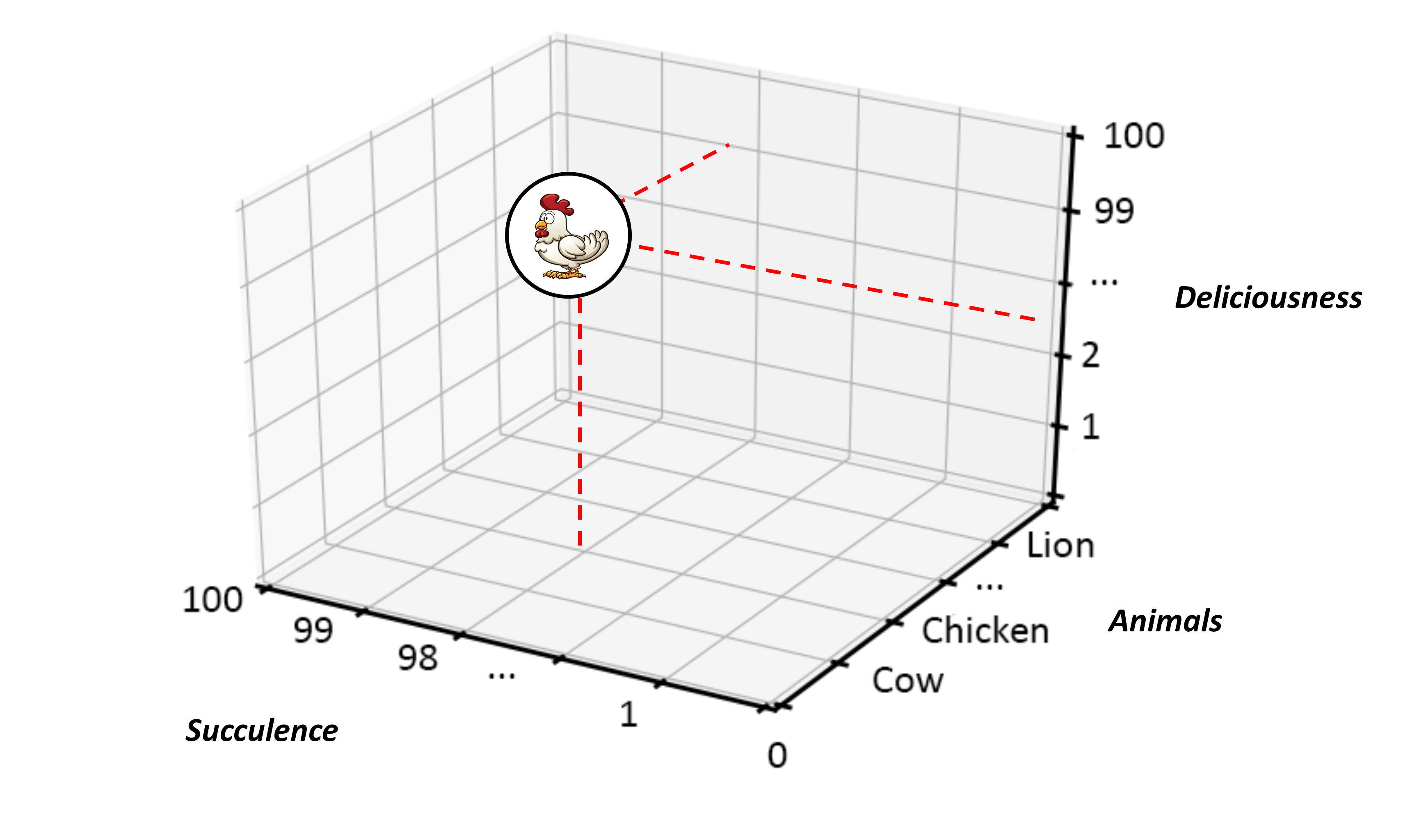
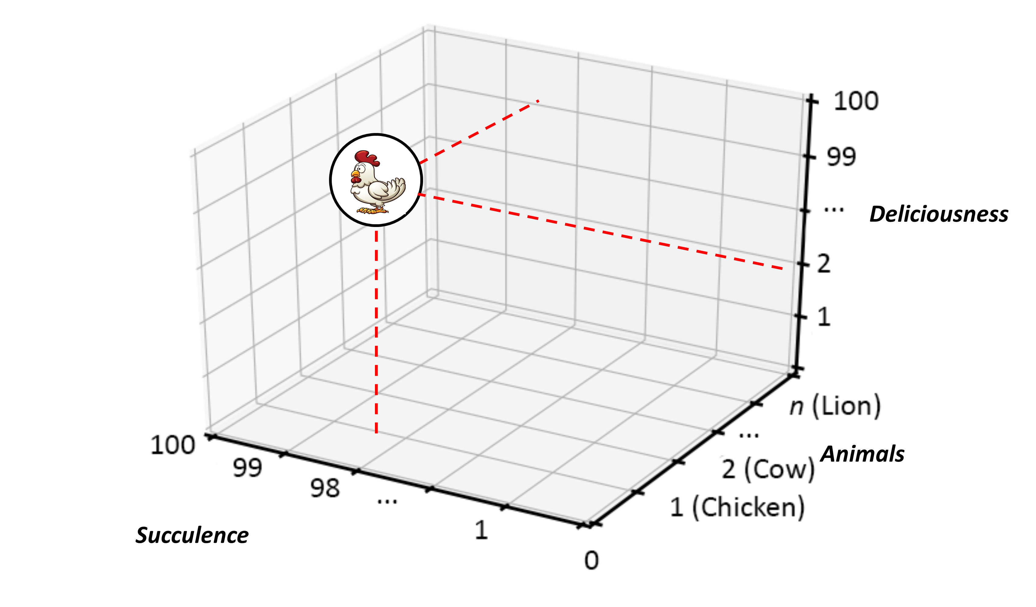
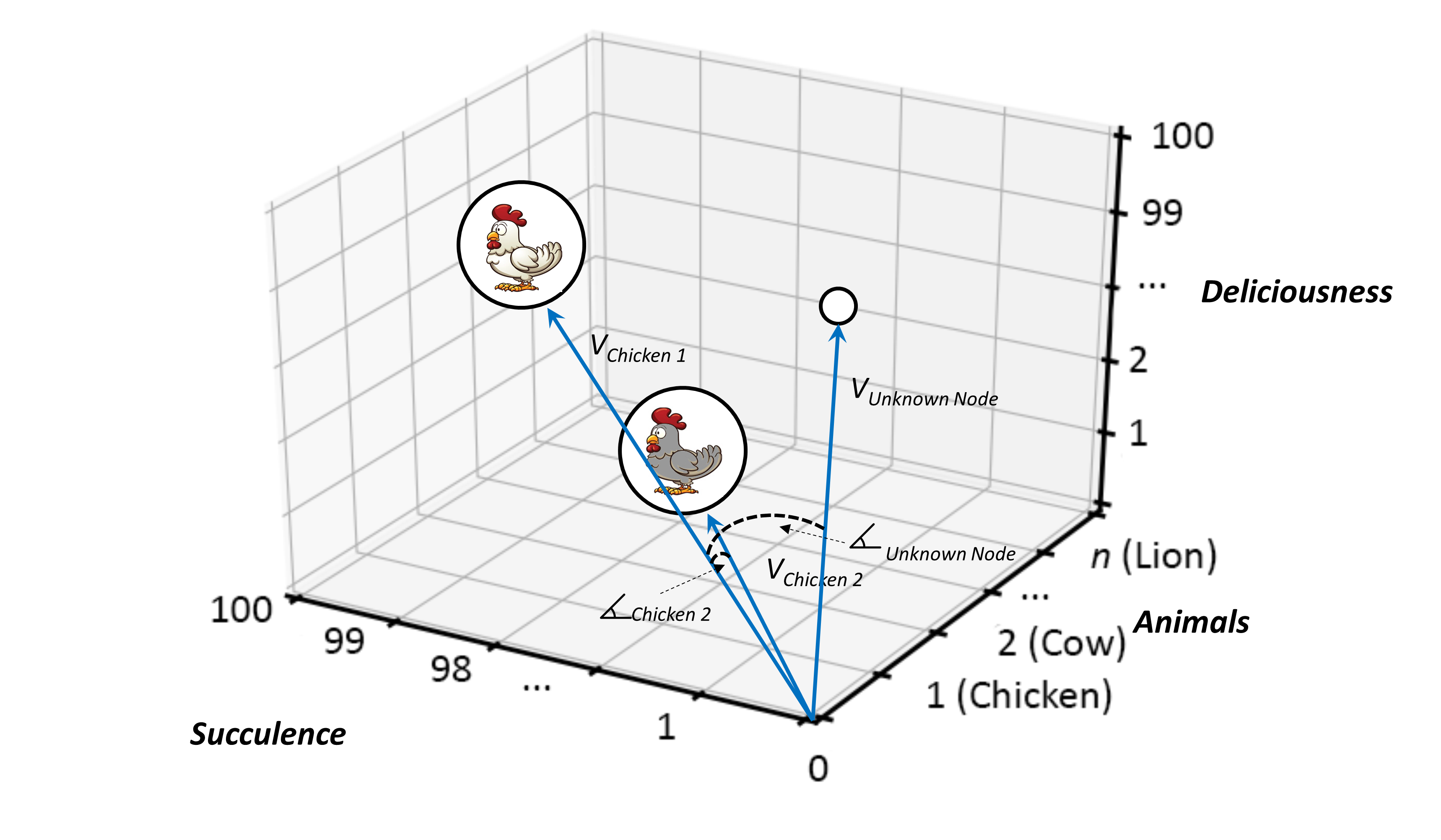
With measurement scales in place for all the features we need to denote — this specific example being Succulence and Deliciousness ascribed to individual Animal:Chicken instances — we can start to think of placing graph structures in a continuously gauged Cartesian space, as shown in Figure 11. This helps us assess (or rather denote) individual Animals:Chickens in terms of their Succulence and Deliciousness. Or perhaps we can think about arranging our list of Animals in alphabetical order and referencing them by their position in that list. That would give a three-dimensional numeric measurement, as shown in Figure 12.
Now things start to get interesting. So, to complicate matters slightly, why not say that we are interested in two instances of Animals:Chicken, rather than one, and suggest that both offer different taste profiles, in which case we might see a representation not dissimilar to Figure 13.
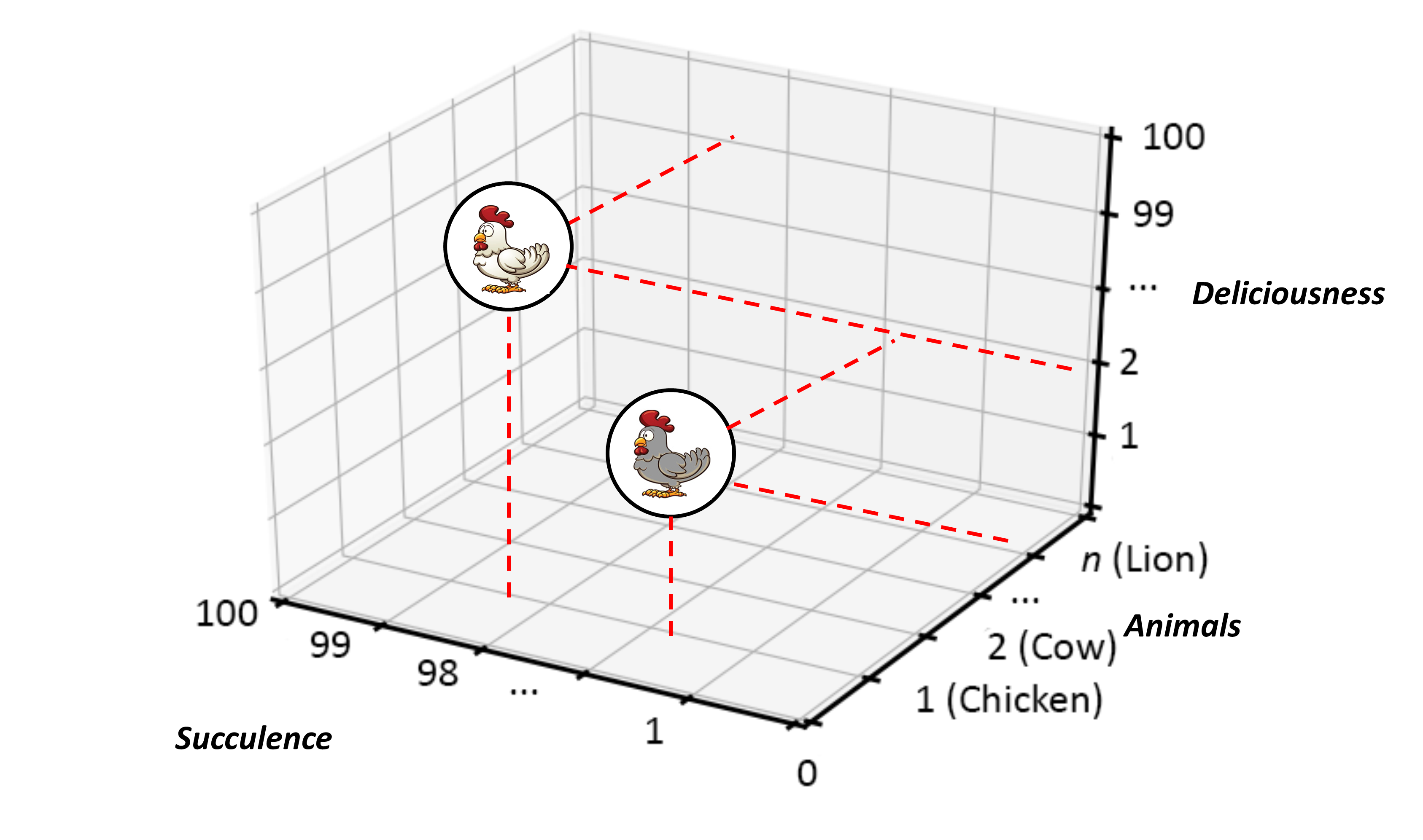
In Figure 13, it should hopefully be clear that both nodes have the same Animals type value of 1, thereby identifying them both as type Chicken, and that both chicken instances possess differing levels of Succulence and Deliciousness. In other words, our two “chickens” may share the same Animal type but do not have the same properties across the board. In this case, that simply implies that they taste different. In that, however, no indication is given as to which tastes better. Betterness, if there is such a thing, is not denoted here, so has no relevance to the context being described. It literally has no meaning.
3.7. Vectors
This scheme is useful because the mathematical measuring schemes imposed by the Animals:Chickens surrounding Cartesian space not only provides a mechanism to denote specific characteristics of interest, but it rather fortunately also provides a way to compare just how different any two Animals:Chickens might be across characteristics.
To make this comparison, the readings from each of the Cartesian axis associated with two Animals:Chickens can be combined into a mathematical system known as a vector, which uniquely identifies the position of each within its surrounding Cartesian space, as shown in Figure 14.
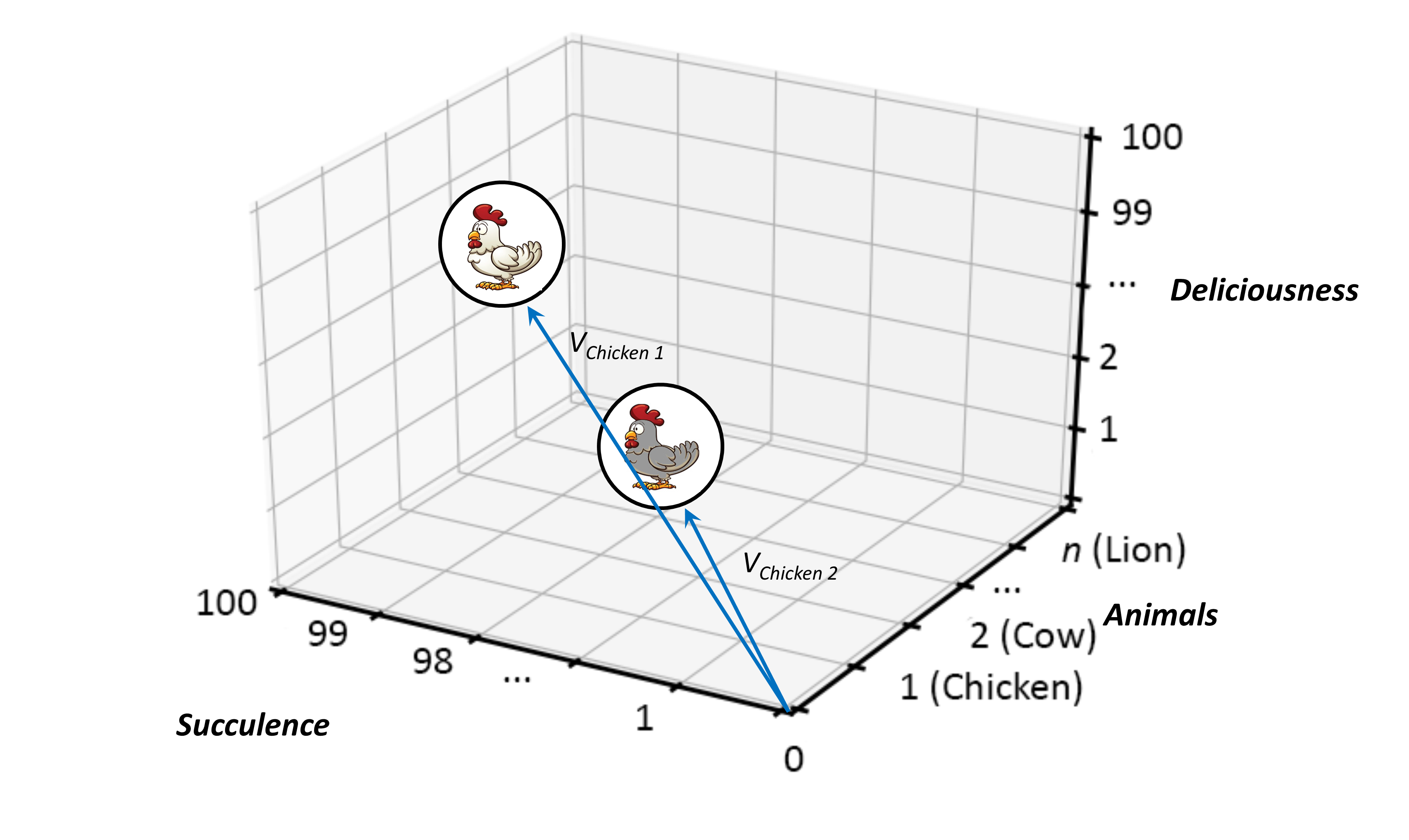
Vectors provide further mathematical advantage here, as they can, given that they contain both magnitude and direction, be used as data structures to store collections of coordinates. As such, they can be mathematically represented using arrays of numbers, where each array element corresponds to a value taken from the axes of any surrounding coordinate space. Similarly, vectors can be represented by a straight line, with its start point conventionally at the origin[7] of its Cartesian system. As a result, when vectors are drawn in such spaces, the space becomes what is known as a Vector Space [77], rather than a Cartesian Space.
3.8. Graph Node Comparison Using Vectors and Trigonometry
When a Vector Space and relevant vectors combine, the resultant framework allows questions to be asked of the things or ideas being represented in vector form and their associated characteristics. In other words, the characteristics of two or more graph nodes can be compared mathematically and with great precision, as shown in Figure 15.
In starting to ask questions, then, the trick is to first forget about a vector’s size for a moment, by temporarily setting it to 1. This then produces what mathematicians refer to as a Unit, or Normalized Vector, and which maintains the same direction as its donor parent. From there on in, comparing any two node locations within a vector space becomes a matter of studying the angle between their respective unit vectors, using the branch of mathematics known as Trigonometry.
Trigonometry, or “Trigs” for short, is one of the basic mathematical staples doled out in school. You remember the drill. It was all about sines, cosines, tangents, and so forth. More formally, though, trigonometry is the branch of mathematics that deals with the relationships between the angles and sides of triangles — particularly right-angle triangles. It is, therefore, used to study the properties of triangles, circles, and other geometric figures, as well as to solve problems involving angles and distances, as we shall do here. The basic concepts of trigonometry include the definitions of the six trigonometric functions: sine, cosine, tangent, cosecant, secant, and cotangent, the relationships between these functions, and their application in solving problems.
That brings us to the outputs provided by these basic trig functions, which are all limited by upper and lower bounds of 1 and -1. With those limits in mind, a mathematical sidestep can next be used to great effect.
If you apply a mathematical modulus function over any trig output — which simply means throwing away any minus sign present — then something rather magical happens. At face value it merely reduces the range of trig output from -1 to 1 to between 0 and 1. Beyond that, however, it miraculously bonds together three highly valuable branches of mathematics. The first we know already, in trigonometry, but what is interesting is that both mathematical probability and continuous logic produce outputs within the same bounded numeric range as the trig-modulus trick we have just played. In that way, trigonometry, probability, and logic map onto the same solution space, meaning that they can all be used to understand the results from the same mathematical test. To say that another way, if you want to know the probability of two nodes in a graph being identical, then you also get the degree of truth associated with that proposition and a route to find the actual angle between the vectors representing both nodes when you apply the appropriate calculation. All are really just mathematical measures of proximity.
This is why the emphasis on John von Neumann’s work early on in this book. Whereas the normally used version of logic, first introduced by George Boole in 1854 and common to most digital computers today, is only interested in the numerical extremes of 0 and 1, von Neumann’s logic is more encompassing and can accommodate the full range of values on a sliding scale between 0 and 1.
You will hopefully recall that George Boole, the mathematician behind Boolean Logic was particular and extreme in his views — stating that logical truth was a discrete matter of all or nothing. In his mind, therefore, a proposition was either wholly true or wholly false. Just like a switch, it was all in or all out, all on or all off. There was no element of compromise in between. Von Neumann, on the other hand, was much more liberal in his position. In his world view, a proposition could be partially true and partially false at the same time. In that way, he considered the world in terms of degrees of truth. Overall therefore, Boolean logic is a subset of von Neumann Logic. Or, in both mathematical and philosophical terms, von Neumann wins. End of story.
In layperson’s terms, this all boils down to the same thing as asking, “How likely is it that something is true?”, such as in the question “How likely is it that that bird flying overhead is a chicken?” Indeed, we might even rephrase that. So, asking “How logical is it that that bird flying overhead is a chicken?”, gives exactly the same proposition as asking “how likely is it?” Chances are that it is not a chicken, so in Von Neumann’s logic that would give us an answer of less than 1/2, but more than 0. In that way, we might, for instance, mathematically reason that there is a 22% chance that the bird is a chicken. Or to rephrase; the probability of the bird being a chicken, based on all known properties and their available values is 0.22. Likewise, it is 0.22 logical that the bird in question is a chicken. Both propositions are mathematically the same. Von Neumann’s continuous logic and mathematical probability behave as if one. Lastly, it turns out that the cosine of the angle between a vector representing a chicken and the specific one that does not in our question, equates to 0.22. That means that the angle between the two vectors is 77.29096701 degrees.
But what are the mechanics of this mathematical love-in? The answer, it turns out, is both mathematically simple and blissfully elegant.
3.9. Cosine Similarity
Cosine similarity [78] is a measure of closeness, or sameness, between two non-zero vectors. Think of it like this: If two identical nodes (points translated into vectors) in any vector space were to be considered, then both would lie at the exact same position within that space — one atop the other. Likewise, they would also possess identical vectors, meaning that both vectors travel along identical paths through the vector space. Identical trajectories also mean that there is no angle between their respective paths, or, more formally, the angle between the trajectories of both vectors is 0 degrees. Now, take the cosine of 0 (zero) and that returns 1 (one), which, in terms of both mathematical probability and continuous logic, corresponds to absolute certainty or truth. In other words, there is complete assurance that both nodes are identical in nature. Or, when thinking in terms of the semantics that both vectors could represent, they carry identical meaning, and, therefore, for all intents and purposes, represent the exact same thing.
Now, consider the opposite extreme, as in when a cosine similarity test returns 0 (zero). Instinctively, it might be assumed that the two vectors being compared represent completely different things or ideas and that is kind of true, but not quite. It means, in fact, that their trajectories from the origin in any given vector space are at a 90 degrees tangent to each other about some particular plane (or set of dimensions/axes), which does give a very specific measure of difference in terms of denotational semantics, but not necessarily a “complete” difference. That is unless it has been externally agreed (denoted) that perpendicular vector orientation does indeed represent full and complete difference. That is because the idea of difference can be subjective, even from a mathematical point of view, as where the idea of absolute similarity is not.
Nevertheless, the use of cosine similarity provides a valuable tool for assessing the proximity of graph nodes, when mapped and measured as vectors in some vector space. It also provides a clear way of understanding just how alike any two nodes are within a graph. And in a complex ecosystem of dynamically changing systems and actors, that is important.
3.10. Bringing This All Together
Right, that is enough talk of chickens and waffles for now. Next, we ground ourselves firmly back in the world of IT architecture and lay down some basic rules for modeling systems in hyper-enterprise contexts. We will state them first, then revisit each in turn to outline why it is important:
-
Document and agree what you know
State the facts and prioritize them in terms of what is important and what needs to be achieved. -
Check and double-check your perspective
Remember that yours may not be the only relevant viewpoint on a problem or solution space. This is especially true in large and complex contexts. What might seem clear to you, could well come across differently to others. As a simple example, think of a sink full of water. To your everyday user, it likely represents no more than a convenience for washing, but to an ant or spider it might as well be an endless ocean. Recognizing that the world is not the same across all vantage points is, therefore, truly important, and accepting more than one interpretation of a situation or thing can often be useful, if not invaluable. -
Schematize what you have documented and agreed
Create whatever tried and tested architectural diagrams you think might be useful and make sure that all relevant stakeholders are bought into your vision. -
Translate your schematics into a generalized graph form
Get to a point of only working with nodes and arcs, with both types properly justified in terms of unique (wherever possible) identifiers, characteristics, attributes, and so on. -
Use your attribute and characteristics to create measurable dimensions (axes) in an abstract vector space
Construct an n-dimensional vector space, where each dimension corresponds to an attribute, characteristic, aspect, or feature needing architectural representation. -
Agree on how vector difference should be defined
Establish guidelines on what types of mathematics should be used to establish vector difference, and how that difference should be measured. -
Embed your graphs into their respective vector space(s)
Translate nodes into n-dimensional vectors and arcs into a separate set of two-dimensional vectors, containing only start-node identifiers and end-node identifiers.
In the case of our original graph example, then, that then gives a pair of vector spaces, as shown in Figure 16.
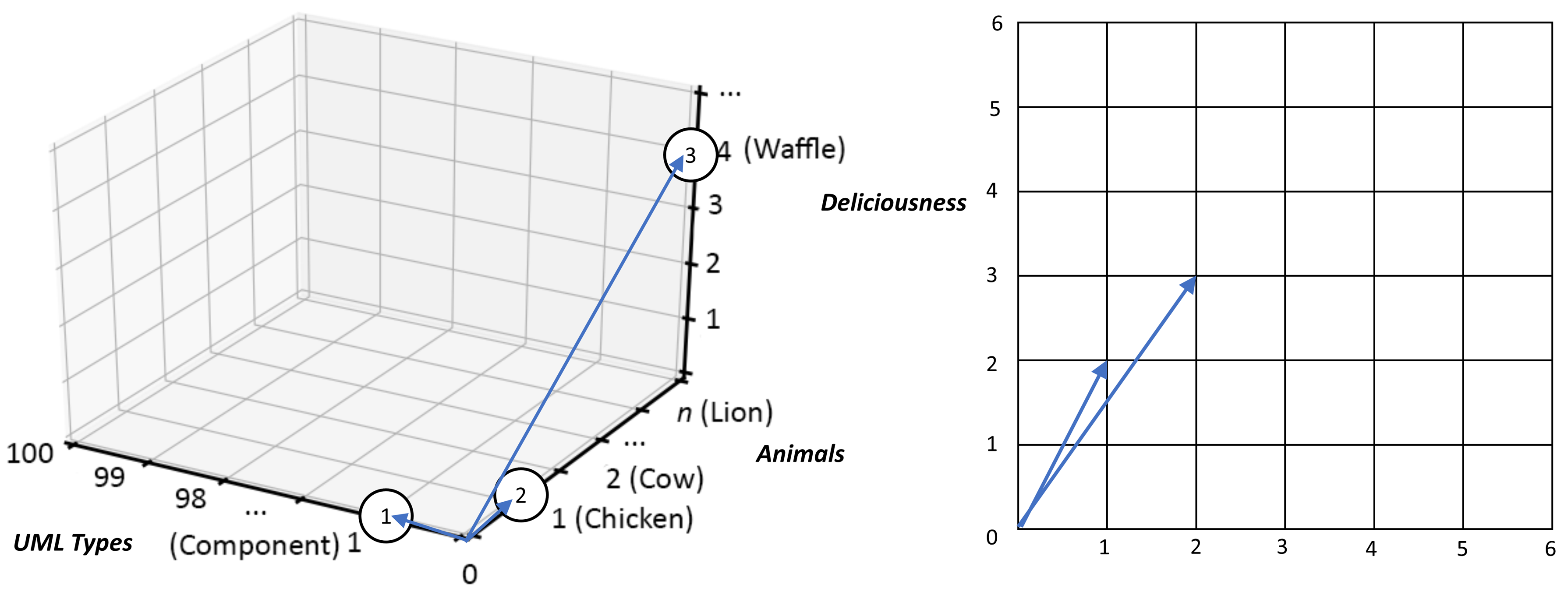
The three-dimensional vector space on the lefthand side of Figure 16 therefore shows the three nodes in our graph and thereby captures each node’s type. This space could, of course, be extended over five dimensions, so that, for instance, degrees of Succulence and Deliciousness might also be included — but in that case the resultant space would be difficult to visualize here. The two-dimensional vector space on the right illustrates how the various nodes in the graph are connected and makes it explicit, for example, that the node labeled “1” is connected to the node labeled “2”. That is via the vector  [8] [79]. Likewise, it further explains that the node labeled “2” is connected to the node labeled “3” — via the vector
  .
.
With both of these vector spaces in place, we now have a way of representing almost all architectural schematics in a graph-based vector form.
3.11. The Value of Vector Spaces in Modeling Ecosystems
By outlining the two vector spaces in the previous section, we have actually covered a lot of ground quickly. First, we have moved the language for architectural expression away from one less formal and open to interpretation — as in the “boxology” of drawn shapes and lines — to one which still accommodates informality of design thinking, but which is much more aligned with precise measurement and unambiguous semantics. Next, we have also found an open-ended way to capture both discrete and continuous measurement. Last, we have overlaid a range of mathematical techniques that can assess important architectural characteristics across the board — not least of which is similarity or sameness.
So far, so good. But now the question is why?
Almost certainly a major difference between classical Enterprise Architectures and hyper-Enterprise Architectural contexts is that ecosystems demand change over time and sometimes that happens beyond the control of the organizations, systems, or participants that they engulf or interact with. In one word, they “evolve”, and that evolution is just as likely to come from agreement en mass, as it is from any single decision or isolated influence. With that, the very idea of hyper-enterprise contexts breeds unpredictability and risk; two things that architects, business executives, and the like generally agree are not good.
But here is the thing. In a graph-based, vector-view of IT architecture, time just becomes one more dimension to consider within the vector spaces in use. So, in a vector-centric world, it therefore is not some extraneous threat, but something that can be accommodated and managed with relative ease. In that regard, it is just one additional mathematical axis (or measurement scale) to be considered. In truth then, by way of vector analysis, time and change actually become an architect’s friend rather than their enemy; immediately affording a way to formally compare the various states of any entity of interest as it plays out its role within some grander ecosystem context. Furthermore, by using techniques like cosine similarity, the implications of time can be rigorously reasoned and perhaps predicted. And that includes risk. If, for instance, the current state of an entity, artifact, property, attribute, or so on is known (through its vector position) and its change history is also understood (through a series of trigonometric calculations), then it becomes a relatively simple analysis task to project out into some future vector plane to guess where the entity’s evolutionary progression might be heading. Likewise, cosine-change-history can be used to help extrapolate out hidden influences driving any such trajectory.
Adding a time dimension can thereby help significantly de-risk hyper-enterprise IT architecture. By the very nature of evolutionary processes, all nodes and arcs in a time-dimensional vector space must be subject to change somehow. This is especially important when thinking in terms of integration. Quite legitimately, what might be presented as a strong and important relationship at one point in time, may well be weakened the next. In simple terms, relevancies may well change, and connections might break or be shown wanting. So, in circumstances where important elements of an architecture fail, how might IT architects look for alternatives?
3.12. Asset Approximation Using Vector Proximity
Here again, a vector-view of IT architecture comes to the rescue. If we look at examples of ecosystems in nature, then a major lesson to be learned explains that perfection is often impractical, if not implausible or even impossible. But sometimes imperfection carries its own advantages. It can lead to serendipity, for instance, one of evolution’s best friends.
The point here is that good enough is often good enough. Cows are equally as able to feast on silage as they are on fresh clover; they simply make do and their species survives regardless. The overall system that is a cow’s lifecycle simply adapts, adopts, and moves on. In short, approximation is good news in the world of ecosystems.
But how does this translate into the hard-nosed world of the IT architect, and our well-drilled practices based on tight conformance to requirements? The simple answer is that, as IT architects, we should, of course, remain focused on the same precise targets as always, but be somewhat prepared to blur their edges. Think of it as appreciating the various outer rings of a bull’s eye’s roundel. Or perhaps better, think in terms of architectural assets having an umbra[9] of definition. That is to say, they have a well-formed core of characteristics that taper off, rather than ending abruptly. Net, net, all hard-edged targets remain, but implanting them into vector-based frameworks opens up the opportunity to surround their boundaries in a blur of tolerable approximation. Absolute must-haves can sometimes, therefore, be translated into close compromises. In vector terms, this simply means that rather than describing a node singularly in terms of its specified dimensional coordinates, architects may consider a region surrounding it as being approximately equivalent. In that way, they can easily search over what they know of a given ecosystem and quickly surface close counterparts in the event of links going down or assets losing their value. Maintaining point-to-point integration then becomes a matter of understanding vector differences and applying fixes so that those differences tend toward zero.
In summary, this is like running a Google®-like [80] query over a complex IT architecture in search of compromise. As such, when things change in an ecosystem, an asset’s surrounding environment can be surveyed to find its closest-possible equivalents or contact points to those in place when the ecosystem was last architecturally sound or stable. Finding closest approximates through multi-dimensional fit-gap analysis, therefore, helps reduce risk and decreases any development effort required to keep up with environmental change. This might feel untried and complex, but it is certainly not the former. The use of “Google-like” was quite deliberate. Google is amongst many web search engines to have successfully used vector-based search methods for years now [81]. Indeed, vector-based search has been a staple of information retrieval research ever since the 1960s [82] [83].
3.13. Star Gazing and the Search for Black Holes
On to one more advantage.
When you ask Google for the details of a local plumber or what the price of milk might be, how do you think it gets its answer back so quickly? Does it throw some massively complex Structured Query Language (SQL) statement at a gargantuan database of all human knowledge? Of course not, not least for the reason that it would take longer to return than Deep Thought required to give its answer of “42” in Douglas Adams’s famous book, The Hitchiker’s Guide to the Galaxy [84]. A long time for sure and easily way longer than any Google user would tolerate. No, of course, it was a trick question. Google does not rely on the eloquent and reliable capabilities of SQL. Instead, amongst many tricks in its box of magic, it uses vector frameworks and vector algebra.
When the Web’s search bots crawl its structure and find a new webpage, they essentially chew it up, spit out the connecting tissue, and weigh up what is left. In doing that, they use techniques similar to those described above, first categorizing worthwhile content then grading it against various category headings. In vector terms, that gives the dimensionality of the web page and a set of measurements that translate into a cloud of points — graph nodes in the form of metered vector end points. These are then indexed and slotted into the grand galaxy of points that is Google’s understanding of the entire accessible World Wide Web.
So, in a very tangible way, when you ask questions of a web search engine it is like staring up at a clear night’s sky. All the Web’s content is mapped out as one great star field of points and connections. Amongst other things, such engines will translate your query into a set of vectors, then cast them out into the night sky that is its understanding. Then all they do is look for stars within the proximity of your query. In essence, they look for overlaps in the umbra of its understanding with that of your enquiry. If and when matches are found, and within tolerable distance, they then count as search results and, barring a few well-placed adverts and so on, the closer the proximity, the higher up the search ranking a result appears. In short, the nearest stars win.
Having said that, this astronomy-based analogy points toward at least one additional benefit for vector-based IT architecture. Believe it or not, search engines like Google, do not and cannot know everything about the Web. For a whole host of reasons, that is just impossible and, likewise, there are not many IT architects in the world who can genuinely claim to know every single detail about the systems that they design and deliver. Again, that is just silly. It is more or less impossible. Parts of the night sky are destined to stay dark, and likewise it is not unusual for regions in a complex IT architecture to be overlooked. Peering into such voids is just a pointless activity.
Or is it?
In many ways, this challenge is like the search for black holes in cosmology. The scientists rarely, if ever, find black holes by staring directly out into the vastness of space. Rather, they apply broad scanning techniques and look for regions where the presence of black holes feels likely. Then they cycle in, each time increasing the level of detail, until they hit or not. In that way, it is not so much the black hole that gives itself up, but rather the context within which it is hiding. This is rather like being asked to describe the shape of a single jigsaw piece without having access to the piece itself. The way to solve this problem is to ask for access to all the other pieces in the jigsaw, then, once assembled, the remaining hole will be the exact mirror image of the piece you seek. Rather than describing it precisely by direct view, you do the same by describing the hole it would leave when taken away from the completed jigsaw. Both descriptions are, therefore, for all intents and purposes the same.
Now, surprise, surprise, a similar trick can be played with Ecosystems Architecture. Once all the facts have been gathered, filtered, and plotted in line with the ideas of vector space representation, then that affords the opportunity to step back and look for unusual gaps. These are the blind spots in IT architecture, the gotchas that every experienced IT architect knows will jump out and bite them at the most inconvenient of times — the gremlins in the works, if you will.
So, might there be a way to help us hunt down these gremlins? Well, when coordinate-based mathematics is in use, as with vector spaces, that is exactly what is available. The mathematical field of homology [85], for instance, essentially deals with this challenge, through the idea of multi-dimensional surfaces — think of the various undulations of a mountain range, but not just in three dimensions. It tries to ask if the various characteristics of such surfaces can be considered as consistent. In two dimensions, that is not unlike putting up two maps in the expectation that a road might be followed from one to the other. If the maps do not cover adjacent terrain or if either or both is wrong in some way, then passage is not guaranteed and clearly there is a problem. Consequently, it is this exact idea of consistency, or rather lack of it, that homology homes in on, and which can be used to seek out “gaps” in multi-dimensional vector spaces. Homology, therefore, allows IT architects to perform the exact opposite of a Google search, by asking what is not present, rather than what is. By looking at the mathematical consistency of an ecosystem’s vector space, for instance, it can pick out jarring irregularities and point the way to the discovery of hidden actors, events, and more besides. This is not only helpful from the point of view of completeness, but also helps regarding essentials like audibility, regulatory compliance, testing, and so on.
This is indeed valuable, as when modeling we, as architects, regularly draw up what we know and want to share. However, we often fall victim to our self-confidence, believing all too often that we have a full understanding, when perhaps we do not. We must always, therefore, make a habit of questioning what we know and what we do not. For instance, is that space between those two boxes we drew on the last diagram deliberate? Is it going to remain open? Will that be forever, or just for now? Was it always a space? These are all valid questions. Indeed, in the case of physical engineering, the idea of voids and gaps has always been critical, not least because of its importance when balancing weight, ensuring structural integrity, and so on. In architectural terms then, we need to take the idea of gaps very seriously indeed and think long and hard about whether they are intentional or not.
3.14. GenAI
As implied, homology can therefore help understand where an architecture or IT system might well be lacking, as and when areas of total darkness are indeed found. These represent zones of missed requirements or bypassed opportunity — areas that are quite literally “off the map”, as it were. They identify matters of potential architectural concern and/or work to be done. They do not, however, necessarily point to a need for human intervention.
The use of the jigsaw analogy above was not coincidental, as it aligns perfectly with the target output of a new type of AI. Known as Generative Artificial Intelligence, or GenAI for short, it aims to automatically extend on the inputs it has hitherto been given; that is, to generate new material beyond that which it has seen.
The recent rush of excitement in ChatGPT [86] provides a great case in point. As a chatbot, it was designed specifically to soak up the Web’s facts, trivia, and happenstance, and then relay it back to interested conversationalists in ways that feel fresh, authoritative, and engaging. So, in essence, that makes it a gargantuan “gap-filler”, designed to augment the knowledge and capability of its users.
Now, admittedly, AI experts are in a quandary about the rights and wrongs of such skill, and also admittedly, GenAIs can be prone to hallucination [87], but when they get things right, the results can be impressive.
But here is the thing. The output from GenAI is not restricted to natural language, as required in casual bot-like exchanges. No, GenAI can output audio, video, and way much more. And not least on that list is program code. So, in a very real sense, it is now becoming plausible to use advanced AI to both find and fill any gaps found in human-designed IT systems, regardless of human-limited restrictions related to complexity and scale.
Furthermore, GenAI is growing in competence and flexibility at an astonishing rate. For instance, several ideas and approaches are already being worked through to equip the foundation models under GenAI with the ability to use external tools like search engines, web browsers, calculators, translation systems, and code[10] interpreters. This especially includes work on Large Language Models (LLMs) in particular aimed at teaching them to use external tools via simple API calls. This thereby not only allows them to find and fill in gaps associated with user input, but also to find and fill in gaps their own ability in autonomic ways.
As of August 2023, examples of ongoing work in this vein can be seen as follows:
-
Tool Augmented Language Models (TALM) combine a text-only approach to augment language models with non-differentiable tools, and an iterative “self-play” technique to boot-strap performance starting from a limited number of tool demonstrations
The TALM approach enables models to invoke arbitrary tools with model-generated output, and to attend to tool output to generate task outputs, demonstrating that language models can be augmented with tools via a text-to-text API [88].
-
Toolformer is an AI model trained to decide which APIs to call, when to call them, what arguments to pass, and how to best incorporate the results into future token prediction
This is done in a self-supervised way, requiring nothing more than a handful of demonstrations for each API. It can incorporate a range of tools, including calculators, Q&A systems, search engines, translation assistants, and calendars [89].
-
LLM-Augmenter improves LLMs with external knowledge and automated feedback using Plug-and-Play (PnP) modules
-
Copilot [91] and ChatGPT Plugins are tools that augment the capabilities of AI systems, like Copilot/ChatGPT), enabling them to interact with APIs from other software and services to retrieve real-time information, incorporate company and other business data, and perform new types of computations [92]
-
LLMs as Tool Makers (LATM) [93] — where LLMs create their own reusable tools for problem-solving
One such approach consists of two key phases:
-
Tool Making: An LLM acts as the tool maker that crafts tools for given tasks — where a tool is implemented as a Python® utility function
-
Tool Using: An LLM acts as the tool user, which applies the tool built by the tool maker for problem-solving
Another lightweight LLM, called the Dispatcher, is involved, which determines whether an incoming problem can be solved using existing tools or if a new tool needs to be created. This adds an additional layer of dynamism, enabling real-time, on-the-fly tool-making and usage.
-
The tool-making stage can be further divided into three sub-stages:
-
Tool Proposing: The tool maker attempts to generate the tool (Python function) from a few training demonstrations
If the tool is not executable, it reports an error and generates a new one (fixes the issues in the function).
-
Tool Verification: The tool maker runs unit tests on validation samples; if the tool does not pass the tests, it reports the error and generates new tests (fix the issues in function calls in unit tests)
-
Tool Wrapping: Wrapping up the function code and the demonstrations of how to convert a question into a function call from unit tests, preparing usable tools for tool users, and so on
The tool user’s role is therefore about utilizing the verified tool(s) to solve various instances of a task or problem. The prompt for this stage is the wrapped tool which contains the function(s) for solving the challenge in hand and demonstrations of how to convert a task query into a function call. With the demonstrations, the tool user can then generate the required function call in an in-context learning fashion. The function calls are then executed to solve the challenge accordingly.
The Dispatcher maintains a record of existing tools produced by the tool maker. When a new task instance is received, the dispatcher initially determines if there is a suitable tool for the task at hand. If a suitable tool exists, the Dispatcher passes the instance and its corresponding tool to the tool user for task resolution. If no appropriate tool is found, the Dispatcher identifies the instance as a new task and solves the instance with a powerful model or even invokes a human labeler. The instances from a new task are then cached until sufficient cached instances are available for the tool maker to make a new tool.
3.15. What Does this Mean for Architectural Practice and Tooling?
Make no mistake, working at hyper-enterprise levels will prove very challenging. Not only will the scale of architectural responsibility and associated workload increase by several factors, but the added vagaries and increases in abstraction involved will certainly be enough to overpower even the most able of IT architects. Furthermore, and as you now know, this sea change in capability leads to the need for some pretty advanced mathematics, and an appreciation for its position in a much broader landscape of deeply theoretical ideas.
Summed up, that is a big ask.
Nevertheless, there is not necessarily any need for concern or despair. As our understanding of IT architecture has improved, so have the tools and technologies within our reach. As already explained, this is an age-old story. As human need moves on, it is so often supported by technological advance. The Industrial Revolution rode on the back of our harnessing of steam power, for example, and likewise, many modern fields of science would not have been possible without the arrival of cheap and plentiful electronic computers. A perfect example can be seen with the relatively recent arrival of Complexity Science. As an undergraduate student at Dartmouth College, Stuart Kauffman [62] found himself staring into a bookshop window and realized that his life would be caught up in the eclecticism of modern science. In that, he marveled at the thoughts of scientific pioneers like Wolfgang Pauli, who had previously remarked that “the deepest pleasure in science comes from finding an instantiation, a home for some deeply held image”. What he was reaching out to would become known as the scientific study of deep complexity, a discipline he would later help establish. Some 30 years on, he had captured its nature in the principles that make physical complexity real. At its peak, he listed life itself as complexity’s greatest achievement and came to understand that physics had to embrace spontaneous chaos as well as order. Somewhere in the middle of both was evolution, and the fact that both simple and complex systems can exhibit powerful self-organization. That much became clear as his work progressed and he teased out the models and mathematics needed. But Kauffman was breaking out at a particularly fortuitous time. To test his ideas through manual experimentation would have proved impossible, as the very thing he was interested in was the same as the stubborn obstacle that had blocked scientific progress in the past, in that complexity feeds at scales well beyond easy human reach. But this time around, Kauffman could sidestep. Personal computers had just become commonplace and were starting to spread across the desks of his academic colleagues. These were more than fanciful calculators, and in the right hands Kauffman knew that they could be deftly programmed to model the aspects of complexity that had stumped his predecessors. In that way, by using modern computing power to augment human skill, Kauffman not only prevailed where others had not, but he blew the doors off previously blocked avenues of investigation. Computer Aided Research had found a sweet spot.
Dial forward to the present day and we find ourselves confronted with a veritable cornucopia of technical capabilities. We have long moved on from personal computers to augment the capability of the individual or group. Today we talk in terms of millions of easily accessible compute nodes, curtesy of the planet’s various cloud compute platforms. Furthermore, we easily measure AI variants, like neural networks, in terms of billions of nodes — increasingly counting even more than in the human brain.
This all boils down to one simple fact: just because a hyper-enterprise problem might be beyond the natural talents of the IT architects assigned to tame it, that does not mean that we do not have the calibre of tooling available to jump the obstacles in place. In fact, it is quite the opposite. To briefly return to our search engine example, companies like Google have harnessed the essentials of vector-based modeling with such success that they now top the list of the world’s most illustrious technical enterprises. So, make no mistake, we have already nailed the application of the highfalutin mathematics involved many times over. Indeed, we now even have a generation of cyber-hungry, phone-clicking millennials who depend upon it. This stuff is so in our face that it is not funny, and we have been ably applying tools and techniques to subdue hyper-headful overflow for decades. That is what modern information retrieval is all about. So sure, it is not beyond the capability of the IT architect community to adopt, adapt, and move on? This will not only push us out beyond the headful, but it will reshape our role in the world forever.
This will happen, make no mistake. Before long, AI-infused IT architecture will be a thing, and likely it will cloak its formidable capabilities behind a façade that will obfuscate the need for any real understanding or appreciation of the scale and complexity playing out behind the scenes. This is what good technology does. It makes the complex feel simple, and that presents an abundance of challenges for professional practice in the future.
Should we allow IT architects to practice without clearly demonstrating their proficiency at the wheel, as well as their understanding of the advanced tools and techniques we are expecting them to drive? If not, what should we teach the next generation of architects to keep them and those in the way of their outcomes safe? Should we allow the intelligence in AI to augment and take the lead, and should we trust its proclaimed ability to assist, rather than hinder or harm? Furthermore, should we slacken our tolerances around professional accreditation in the same way that we are advocating the widening of focus — to embrace umbral appreciation — at the ecosystems level? These are moral and professional questions that will need to be worked through, but certainly, the tools and techniques needed to help the jump to Ecosystems Architecture are very real and with us now. All that is really needed is an increased awareness amongst the global IT architect community and continued endorsement from various accrediting bodies, like The Open Group.
This position is further supported by a generation of new technologies, already perched on the horizon.
The ideas behind quantum computing may seem alien and new, but actually they are neither. Classical computers, or digital computing machines as they might be more correctly labeled, actually make up a subset of all possible ways to compute, and, as such can be seen as part of a much broader class of computers, which included quantum devices. All electronic switches are partially quantum-like in their makeup, for instance. For all that we usually consider such devices to be in either an on or off position, by virtue of the electrons flowing across them, when in the act of switching, there must come a point where a switch’s last few electrons are in transit between a its two poles. So, in that miniscule moment, the switch is neither on nor off, and it is extremely hard to ascribe which of the two positions is most relevant. This is one small step removed from the very essence of the quantum world, in the idea of super position — the fact that quantum systems can be seen to be in multiple states all at once. And to describe this super-class of switching capability, it is no coincidence that vector-based mathematics is used. In the world of quantum mechanics, the abstract vectors we have labored so hard to describe here actually carry a special name. In that world, they are known as eigenvectors — after the German term meaning “own”, and which is a good way to think of values or vectors that are “characteristic” in one way or another. Likewise, quantum mechanics relies heavily on the idea of probability to consider how superposition might change over time[11] into an identifiable state once inspected; this is just the flip side of a coin that also features continuous logic. All mix together into the same mathematical framework as we have previously described, and all are essential to penetrate the microscopic world below the reach of human experience.
Is this just coincidence? Is it some joke at the expense of those who do not understand the overlap between high-end mathematics and science? Absolutely not. There is a key phrase in the paragraph above, in the “reach of human experience”. Both the subatomic and the hyperscale are exactly that. They are unprobeable by any direct human means of interaction or inspection. Yet still, we know that both exist and are very much of our world. What we cannot do, however, is consider them as being humanly tractable, simply because their manifestation lives beyond the realm of direct human experience. One is firmly below us, while the other firmly above.
With all options to assess human-level relatability removed, we are then only left with one option. All that remains is our appreciation and understanding of the abstract and the uncertain, as how can we possibly ascertain any ground truth without help to augment our insight. This is like Neanderthal man learning to mine an anthill for protein with a stick, or ancient warriors favoring iron weaponry over bronze. In the same way, the invention of the microscope opened up much of modern medicine and likewise 20th century breakthroughs in philosophy led to the birth of the modern-day computer. Sticks, microscopes, and digital computers are all just tools, as are the various formulations of mathematics. All have been, and will be applied, to get a handle on what we cannot appreciate directly. Where the timing of events is uncertain, then mathematical probability becomes the weapon of choice, just like the box and the line are the IT architect’s weapons of choice on our traditional battlegrounds today. Likewise, abstract vectors point the way to understand what can only be contemplated in imaginary terms. There is no real difference. Box, line, probability, vectors. Simply pick your tool and step forward. A job of work needs to be done.
Likewise, at higher levels of abstraction, it is possible to think of additional suites of mathematics brought to help understand how Ecosystems Architectures might behave over time. Here, tools like mathematical Game Theory [94] and Monte Carlo Analysis [95] come to mind, but the key thing to remember is that, just like graph theory and vector analysis, they amount to nothing more than tools to help understand that which we cannot face head-on. Whole other chapters could be written on how and how not to apply them at hyper-enterprise levels, but there really is no need. The techniques listed above provide a framework for representation and can thereby hopefully act as a foundational layer over which additional tooling might be applied.
3.16. Limitations and Inference
Because of their inherent flexibility, graphs can model most things, but not all. This becomes especially clear when context-based conditionality is involved.
To illustrate, let us contemplate the relationship between ice and water. When considered from the perspective of their chemical composition, both are identical and can therefore be represented via a graph triple, as shown in Figure 17.
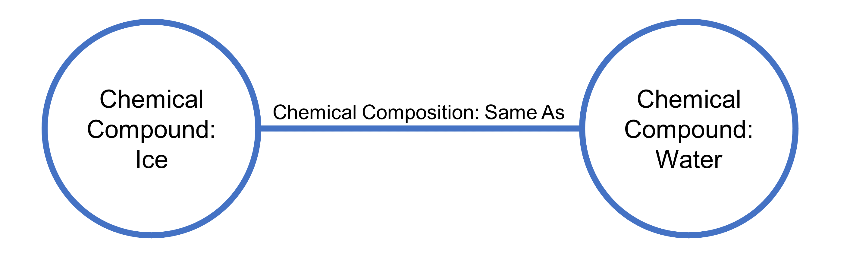
From a physical perspective, however, ice and water are obviously very different, with one being a solid and the other a liquid. On that basis then, the graph shown in Figure 17 could be extended to model the physical deltas in place. But that is all it would do. In that, it would capture the essence of the two physical states. What it would not do, however, is capture the conditions under which hydrogen and oxygen combine to give either water or ice. In simple terms, it would not capture the rules covering the creation or destruction of any state being modeled. In that sense then, graphs are good at recording statements about an individually named situation, thing, or idea, but are not so good at capturing how or why such statements might be seen as real, relevant, or valid.
Notice the word “statement” in the previous paragraph. It is indeed apt, as all that graphs really allow you to do is capture some essence of an individual state, being, or relevance. Any essence associated with transition or conditionality around those things must, therefore, be overlayed using some other technique — as we did earlier by using vector coordinate systems to perhaps model dynamic behavior over time. You can, of course, document any such rules as attributes alongside the nodes or arcs in a graph, but to understand and use those rules, their location and purpose would need to be made clear. And, as those instructions would be external to any graph, or graphs, involved, they too must be considered as an overlayed system.
Attempts have, however, been made to create graph specification languages specifically aimed at bringing denotational semantics and contextual rule systems together. For example, the Semantic Web Rules Language (SWRL) [96] [97] was developed under the auspices of the World Wide Web Consortium (W3C®) Semantic Web initiative [98] [99] in 2004. That was founded on Description Logic (DL),[12] [100] but suffered take-up challenges due to its abstract nature and problems with formal decidability [101].
Having said all that, and although rules inclusion is not hard-baked into the idea of graphs (or graph-based languages) directly, some very useful types of logic lie very close to graph theory. Inductive reasoning, or inferencing [102], for instance, is a key feature of graph-based modeling, which gives “the derivation of new knowledge from existing knowledge and axioms” [103], like those represented in a graph format by way of nodes and edges.
To understand this better, think of the fictional character Sherlock Holmes [104]. He used deductive powers to set him apart as the preeminent detective of Victorian London, taking known facts from his cases and related them to his encyclopedic understanding of crime and criminal behavior. That allowed him to discover new relationships between his foe and what he already knew about crimes and criminals. In a nutshell, that is inference.
As a specific example, consider these two facts about the ancient philosopher Socrates:
-
All men are mortal
-
Socrates was a man
From these it is possible to infer that Socrates was mortal and, therefore, either that he is dead or will die some day. None of these things have been explicitly stated, but they are eminently sensible based on what limited information has been provided. In a similar vein, it is possible to infer that two services interface together if specifics of their data exchange are given, even if a definitive declaration of integration is not.
3.17. GenAI Patterns for Ecosystems Architecture
All of this is leading to an interesting tipping point. As the pace of change accelerates in areas like GenAI, it is becoming increasingly plausible to use synthetic help to augment and automate architectural practice. For instance, LLMs, such as those used in Retrieval Augmented Generation (RAGs) patterns [105] are becoming more proficient by the day and many persist, retrieve, and process their data using vector-store databases. An example is shown in Figure 18[13]. These use the exact same mathematical techniques labored over in this chapter. To begin with, that means that there is an immediate and direct affinity between LLMs and the architectural methodology laid out here. In other words, it is eminently feasible, and indeed sensible, to sit LLM chatbot facilities alongside any knowledge-graph(s) created from an ecosystem site survey. In that way, once architectural thinking has been encoded into graph form, it can be embedded into a vector system and used to directly train some of the world’s most advanced AI — ultimately meaning that practicing architects can interact with massive-scale, massively complex hyper-Enterprise Architectures in a very human, conversational way and well above the level of a single headful.
By adding features for homological analysis, such LLMs can also not only understand the architectural detail surveyed but also what is missing. This is game-changing, as when questions are asked of an architecture, its attached LLM(s) can ask questions back to help automatically fill in gaps and extend existing knowledge. This moves the chatbot exchange on from a one-way question and answering flow, to a genuine two-way conversation. That both increases awareness and scopes out any need for functional extension by the LLM itself.

Semantic rule systems can also be overlaid to help establish context when training or tuning LLMs. This is equivalent to providing an external domain-specific grammar and helps cast differing worldviews down onto whatever knowledge is in place. In analogous terms, this generates guide rails to tackle ice-water-like problems, such as the one described earlier.
Finally, conversation workflows can be applied. These help govern the sequencing of LLM interactions and also filter out dangerous or inappropriate exchanges. For instance, an architect might ask about the specifics of a flight control system, without being appropriately qualified or cleared to do so.
Of course, all reasoning, inferencing, and gap-filling must be architecturally sound. And that is where the human element comes back into the equation. Sure, an LLM-based GenAI might, for instance, be able to ingest previously written program code in order to document it automatically — thereby saving development time and cost — but ultimately and rather amusingly perhaps, this points to some whimsical wisdom once shared by the famous author Douglas Adams. In his book, “Dirk Gently’s Holistic Detective Agency” [106], Adams laid out a world in which everyone has become so busy that it is impossible to meaningly sift through the amount of television available. As a result, inventors have developed an intelligent Video Cassette Recorder (VCR) which can learn what programs viewers like and record them spontaneously. Even better, as these machines are intelligent, they soon work out that humans no longer have time to watch television at all. So, they decide to watch it instead, then erase the recording afterwards to save humans the bother.
3.18. So What?
This all leads to a big “so what?”
Hopefully, the primary challenge is clear, in that there is a very real opportunity to take AI too seriously and too far. That is why human judgement must always, always be kept in the loop. Beyond that, there is just more and more data coming at us and in more and more ways — from more processing, more sensors, and increasingly more data created about data itself. The list just goes on and its growth is beyond exponential. What is more, now, with the growing potential of the new AI-on-AI echo-chambers before us, yet more data will surely be added to the tsunami. As a result, we humans will simply run out of time and options to consume all the information that is important. So, how can we make sure we stay in the loop for the essential intel? How do we navigate in a world of overflowing headfuls? This is surely a problem for us all, but more so for us as architects.
This also obviously raises significant moral, ethical, and professional challenges, but also, ultimately, further highlights an inevitable paradox: we cannot progress without some form of external, almost certainly artificial help, while, at the same time, that help threatens to undermine the very tenets of professional practice and, dare we say it, excellence. For instance, what if we were to use GenAI to create both our architectural designs and the spewing code they demand to create the IT systems of the future? More profound still, what if we were to use AI to help drive out architectural standards? These possibilities have both now crossed the horizon and are increasingly within reach. Exciting, maybe. Dangerous, potentially. World-changing, almost certainly.
In short, we urgently need to find ways to monitor, learn from, account for, and limit the AIs we choose to help augment our world. But how we do that is, as yet, unclear. Control over individual AI instances will likely be untroublesome, and, sure, general rules, regulations, and laws can be laid down over time. But what about the network effect? What about muting the echoes from the world-wide AI echo chambers that will surely emerge. Imagine an AI equivalent of the World Wide Web, with billions of connections linking millions of small and apparently benign AIs — all feeding on the human thirst for more and more data, more stimulus… more help and, perhaps, more servitude and adoration? Make no mistake; this is the potential for swarm intelligence beyond ad nauseam. It is what the author Gregory Stock once referred to as “Metaman” [107] — the merging of humans and machines into a global super-organism. Or perhaps even the technical singularity first prophesied by John von Neumann himself, back in 1958, and in which all we will see is a “runaway reaction” of ever-increasing intelligence.
In truth, we are seeing this already at low levels, by way of the Augmented Intelligence already emergent through the World Wide Web of today. World-wide awareness of news and global affairs has risen for the better, for instance, as has open access to education. But so too has the speed at which radicalization and hate crime can spread. So, what we have the is a double-edged sword that will surely only cut deeper if we tip over from augmentation headlong into a reliance on that which is fully artificial.
And who will protect us against that? Who are the guardians? Where are the Jedi when we need them?
Some would argue that it is us, the IT architects who hold the AI genie’s bottle for now. Can we even stop the cork from popping? This is but one of the profound questions we must face as the age of Ecosystems Architecture dawns.